Prior Distribution: Simple Definition, Example

A prior distribution represents your belief about the true value of a parameter. It’s your “best guess.” One you’ve done a few observations, you recalculate with new evidence to get the posterior distribution.

Formally, the new evidence is summarized with a likelihood function, so:

Posterior Distribution = Prior Distribution + Likelihood Function (“new evidence”)

How Do I Create a Prior Distribution?

You could just take your best guess and sketch some kind of probability distribution (with a few descriptive parameters like the mean or the standard deviation).

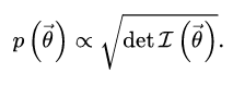
If you don’t have any clue about what the distribution should look like, then you use what’s called an uninformative prior (or Jeffrey’s Prior). It’s exactly what is sounds like and is equivalent to picking a distribution out of a hat. Even if your model is completely unreasonable, once you’ve made some observations your posterior distribution will be an improvement over your initial guess. In fact, an uninformative distribution has very little effect on a posterior distribution, compared to a known prior.

More formally, those guesses at parameters are called hyperparameters— estimated parameters that do not involve observed data. Hyperparameters capture your prior beliefs, before data is observed (Riggelsen, 2008).

Calculating a prior distribution is the easy part. The stumbling block is turning that prior distribution into a posterior distribution. Incorporating prior beliefs into a probability distribution isn’t as easy as it sounds. One option is the Metropolis-Hastings algorithm, which can create an approximation for a posterior distribution (i.e. create a histogram) from the prior distribution and any observed samples.

References

Riggelsen, C. (2008). Approximation Methods for Efficient Learning of Bayesian Networks. IOS Press.