Post Hoc Tests > Duncan’s Multiple Range Test
What is Duncan’s MRT?
When you run Analysis of Variance (ANOVA), the results will tell you if there is a difference in means. However, it won’t pinpoint which means are different. Duncan’s Multiple Range test (DMRT) is a post hoc test to measure specific differences between pairs of means. To learn more watch the video below or keep reading.

Can’t see the video? Click here to watch it on YouTube.
Duncan’s Multiple Range Test was originally designed by David B. Duncan as a higher-power alternative to Newman–Keuls. DMRT is more useful than the LSD when larger pairs of means are being compared, especially when those values are in a table. DMRT tends to require larger differences between means compared to the LSD, which guards against Type I error. For example, while the LSD might say a difference of means of 6 is significant, the DMRT value might be double that, guarding against the possibility of marking differences significant when they are not.
Technology is usually used to find values for DMRT. By hand, the procedure is essentially the same as that for Fisher’s LSD. The main difference is that instead of looking up the critical value in a t-table, you would look in a q-table.
Duncan’s Multiple Range Test Example
Note that this test assumes you have run ANOVA and have a significant result.
Calculate DMRT for the following output:
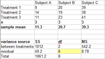
Step 1: Rank the treatments from highest to lowest mean. For this set of data, the means in order are:
- 39.3
- 20.7
- 11.3
The next few steps are to compare the highest mean (39.3) with the lowest (11.3) mean, which have a difference of 39.3 – 11.3 = 28.
Step 2: Look up the q value in this table. With 3 treatments, and 6 degrees of freedom for the error term, the Q value is 4.34 .
Step 3: Find σd2.
σd2 = 2 x residual mean square / n = (2 * 8.78) /3 = 5.85
Step 4: Take the square root of Step 3:
σd = √5.85 = 2.42.
Step 5: Multiply σd (Step 4) by the q-value (Step 2):
2.42 * 4.34 = 10.5.
The difference between the highest and lowest means is greater than 10.5, so the highest mean is significantly different from that of the lowest mean.
The next few steps are to compare the second highest mean (20.7) with the lowest (11.3) mean, which have a difference of 20.7 – 11.3 = 9.4.
Step 6: Look up the q value in this table. With 2 treatments (you are excluding the highest mean now, so the q-value will change), and 6 degrees of freedom for the error term, the Q value is 3.46.
Step 7: Multiply σd (Step 4) by the new q-value (Step 6):
2.42 * 3.46 = 8.37.
The difference between the second highest and lowest means is greater than 8.37, so the second highest mean differs significantly from that of the lowest mean.
If you have more values in your table, continue down your table, changing the q-value as you go. Once you have a non-significant result, you can stop at that point.