Probability Distributions > Truncated Normal Distribution.
What is a Truncated Distribution?
A truncated distribution has its domain (the x-values) restricted to a certain range of values. For example, you might restrict your x-values to between 0 and 100, written in math terminology as {0 > x > 100}.
There are several types of truncated distributions:
- Truncated from above: high values of x are cut off so your range is from negative infinity to some maximum value of x {-∞,xmax}.
- Truncated from below: low values of x are cut off so your range is from some minimum value of x to positive infinity {xmin, ∞}
- Double truncation: both the low values and x values are cut off {xmin, xmax}.
- If values range from negative infinity to infinity {-∞, ∞}, there is no truncation.
Truncation happens when datasets have values that are outside of a usual range. Let’s say you wanted to study income data for the first 1,000 people who submitted census forms. As you’re only studying the first 1,000 people, any income data you calculate would be truncated.
The Truncated Normal Distribution
The truncated normal distribution is defined in the same way as the normal distribution: by the mean(μ) and standard deviation(σ). You’ll also choose a range to limit the distribution to an upper, lower or double truncated distribution. So for these distributions, you’ll have four parameters:
- μ: the mean.
- σ: the standard deviation.
- a: the lower x-value (can be as low as -∞).
- b: the upper x-value (can be as high as ∞).
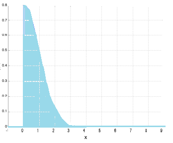
The following normal distribution has had the x-values restricted from 0 to ∞ (a lower truncation), giving the probability density function(pdf) of just half the normal curve:
You’ve probably used truncation without even realizing it; in elementary statistics classes, the normal distribution (and accompanying z-tables) are often truncated to 3 standard deviations around the mean. But the empirical rule tells us that while 99.7% of data does tend to fall within that boundary, there’s 0.03% of the data that falls somewhere outside (there could be the oddball value that’s 10, 20, even 100 standard deviations away from the mean! Truncating allows us to deal with the bulk of the data in a reasonable way.
Mean of the Truncated Distribution
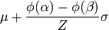
The mean of the truncated distribution is almost impossible to find by hand, because you need to calculate the pdf of the normal first. You’ll want to use software–most statistics packages can handle these calculations. W. Joel Schnedier has created a handy Excel spreadsheet on their Wordpress blog to find the mean and standard deviation of a truncated distribution. You can download the spreadsheet here.
References
Caspeele, R. (Ed.) (2018). Life Cycle Analysis and Assessment in Civil Engineering: Towards an Integrated Vision. Proceedings of the Sixth International Symposium on Life-Cycle Civil Engineering (IALCCE 2018), 28-31 October 2018, Ghent, Belgium.