Differential Equations > Separation of Variables
Separation of Variables is a standard method of solving differential equations. The goal is to rewrite the differential equation so that all terms containing one variable (e.g. “x”) appear on one side of the equation, while all terms containing the other variable (e.g. “y”) appear on the opposite side.
Ordinary Differential Equations
Let’s take a look at an ordinary differential equation:
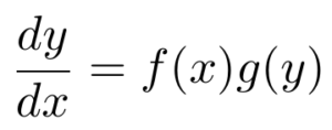
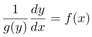
In this unique example, the functions f and g each depend on just one variable. With this condition satisfied, we can now “separate” the expressions related to x from the expressions containing y. To accomplish this, we can rewrite the equation so that the functions f and g are on opposite sides. First, divide by g(y):
Next, multiply both sides of the equation by dx.
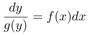
Now, the equation is structured such that all terms related to y are on the left-hand side, while all x related terms are on the right-hand side. So, we can now integrate both sides of the equation.
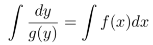
The differential equation can now be either analytically or numerically solved, depending on what functions are actually in the equation.
Practical Example
For practice with the separation of variables technique, let’s consider the differential equation below:
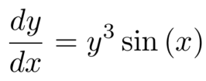
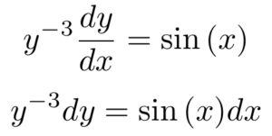
Looking at this ordinary differential equation, we can see that it fits the form for separation of variables because the terms with y and the terms with x can be “separated” on opposite sides of the equation. Like we did in the example, let’s rewrite the equation to isolate all y terms on the left-hand side of the equation, leaving x terms on the right-hand side.
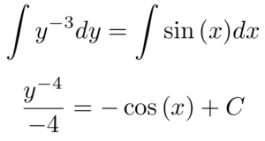
We can now integrate both sides. For the left-hand side of the equation, we’ll use the power rule for integration since we have a polynomial function. The right-hand side becomes negative cosine, the anti-derivative of sine, plus an unknown constant, C.
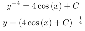
The result is an equation that represents all solutions to our original differential equation example, where C represents an arbitrary constant. Sometimes, we want to write an equation that isolates y on one side. We can do this with our example function:
Separation of Variables: Partial Differential Equations
Beyond ordinary differential equations, the separation of variables technique can solve partial differential equations, too. To see this in action, let’s consider one of the best known partial differential equations: the heat equation.
The heat equation was first formulated by Joseph Fourier, a mathematician who worked at the turn of the 19th century. At that time, the very concept of differential equations was only in its infancy. Accordingly, Fourier’s hypothesis was slow to catch on.
Fourier postulated that the rate at which temperature changes in a solid is proportional to the diffusion of heat across that solid.
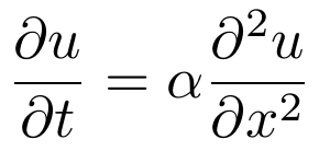
For example, if the heat were spread evenly across the solid, then temperature change over time would be zero. In contrast, if a massive influx of heat were to come from a region in the solid, the temperature of nearby areas would quickly increase.
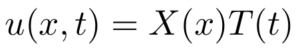
Let’s use the separation of variables technique to break down the heat equation into ordinary differential equations, which are easier to manage. To do this, we’ll have to use a particular method called “ansatz.” An ansatz, a Greek word meaning “guess,” can help us arrive at a solution. It just so happens that with the heat equation, the correct ansatz is a separable function (Hancock).
Substituting this ansatz into the partial differential equation, we have
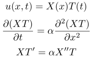
At this point, we can again separate the expressions that contain only x from those that contain only t.
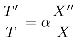
Next, I will claim that either side of this equation must be constant. While this may seem surprising at first, think about the fact that the two sides do not share any variables. In other words, changing the value of t only affects the left-hand side of the equation. Similarly, maintaining the value of xwill only affect the right-hand side of the equation.
So, we can write that both equations are equal to some constant, k.
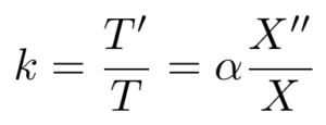
This step is critical because now the original partial differential equation can be broken down into two ordinary differential equations, each equal to a constant,k.
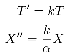
The advantage of separating our equation in this way is that now we can take full advantage of the various methods for solving ordinary differential equations. After all, there are many more of these than ways to solve a partial differential equation.
Ultimately, the separation of variables technique is a relatively simple analytical method, but it can be powerfully applied to both ordinary and partial differential equations.
Legendre Function
A Legendre function is any solution of the Legendre equation.
Where Does The Legendre Equation Appear?
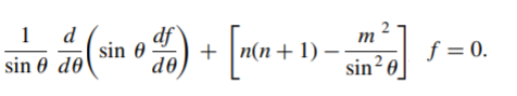
Legendre equations (and their solutions) appear in electrostatic problems, wave functions for atoms, and many other applications. When separation of variables is used to solve a scalar wave equation in spherical coordinates, the following associated Legendre equation arises:
Substituting cos(Θ) = x gives:
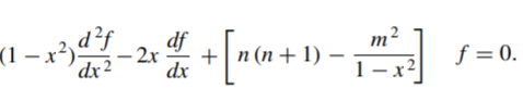
If m = 0, the above equation reduces to the ordinary Legendre equation:
Legendre functions of the first and second kinds are solutions to this equation (Misra, 2007).
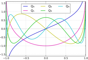
Legendre Function: Types
There are two types: first kind Pv(z), and second kind Qv(z). Both types are linearly independent solutions to the ordinary Legendre equation.
- The Legendre Function of the First Kind is a solution to the Legendre equation.
- The Legendre Function of the Second Kind is also a solution to the equation, except that the solution is singular at the origin.
Calculation
Calculating the Legendre function is usually performed with software. For example, this online calculator from Casio will calculate both Pv(z) and Qv(z) with just two inputs: a value for z and a specified degree.
References
Abramowitz, M. and Stegun, I. A. (Eds.). “Legendre Functions.” Ch. 8 in Handbook of Mathematical Functions with Formulas, Graphs, and Mathematical Tables, 9th edition. New York: Dover, pp. 331-339, 1972.
Misra, D. Practical Electromagnetics: From Biomedical Sciences to Wireless Communication. Wiley, 2007.
Morse, P. M. and Feshbach, H. Methods of Theoretical Physics, Part I. New York: McGraw-Hill, pp. 597-600, 1953.
Snow, C. Hypergeometric and Legendre Functions with Applications to Integral Equations of Potential Theory. Washington, DC: U. S. Government Printing Office, 1952.
Separation of Variables: References
Hancock, Matthew. The 1-D Heat Equation. 2006, https://ocw.mit.edu/courses/mathematics/18-303-linear-partial-differential-equations-fall-2006/lecture-notes/heateqni.pdf.
Narasimhan, T. N. “Fourier’s Heat Conduction Equation: History, Influence, and Connections.” Reviews of Geophysics, vol. 37, no. 1, Feb. 1999, pp. 151–72. DOI.org (Crossref), doi:10.1029/1998RG900006.