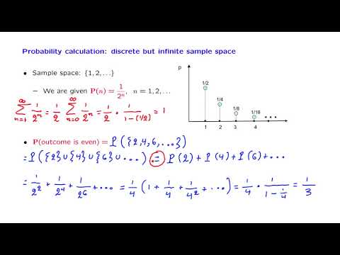
The countable additivity axiom states that the probability of a union of a finite collection (or countably infinite collection) of disjoint events* is the sum of their individual probabilities.
In other words, given an infinite sequence of disjoint events A1, A2, A3, … then their total probability is:
P(A1, ∪ A2 ∪ + A3 ∪ …).
*Note: Disjoint events can’t happen at the same time; They are mutually exclusive with an intersection of zero.
Formal Definition of Countable Additivity
The countable additivity axiom can also be stated as(Nandori, 2012):
If {Ai: i ∈ I} is a countable, pairwise disjoint collection of events, then:
![]()
Where ℙ is a probability measure (or probability distribution) for a random experiment and Σ is summation notation (which means “to add up”).
A function that has countable additivity is called a countably additive function.
Why Do We Need Another Axoim?
For a detailed explanation of why the axiom is necessary, watch this excellent video by MIT Professor John Tsitsiklis. Or, read on below for a brief overview:
This axiom is almost identical to the probably axiom for disjoint events you may have come across in elementary probability: The probability of two or more disjoint events is the sum of their probabilities. Although that rule works for the majority of cases, it does come with an apparent paradox.
As an example, consider a sample space of a unit square, made up of an infinite number of single points.
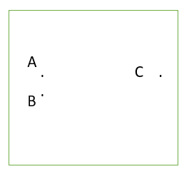
We know from elementary probability that the probability of the entire area is equal to 1 (i.e. the area of the unit square). Now let’s consider the probability of a single point like A, B, or C: The probability of one of these elements happening is zero, so the union of all these tiny elements (A + B + C + …) is also zero. This leads to a paradox, because we have just proved that 0 = 1.
The introduction of the countable additivity axiom removes this paradox, because it states the elements must be a countable sequence of events. The unit square shown above isn’t countable (i.e. it’s elements can’t be placed in a sequence).
References
Haberman, S. (1996). Advanced Statistics: Description of Populations · Volume 1. Springer.
Nandori, P. (2012). Retrieved October 5, 2020 from: http://math.bme.hu/~nandori/Virtual_lab/stat/prob/Probability.pdf