Before you can solve for the area under a normal curve, you must be able to imagine what the area looks like. The best (albeit optional) way do this is to make a sketch. For example, let’s say you were give a z-score and were asked to find the area between that score and z = 0 (the mean). Your sketch might look like this:
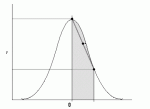
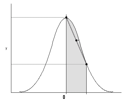
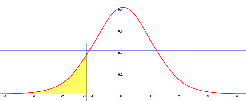
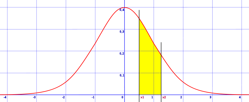
There are seven ways your sketch could look, depending on what z-values you were given. Once you have drawn your sketch, look at the pictures below. Click on the image that looks most like your sketch. The link will take you to a step-by-step guide on how to find the area under a normal curve for that shape. Many of these also have short videos showing the steps.
This video shows you how to find the area under a normal curve for a tail (either a left or right tail):
Choose One
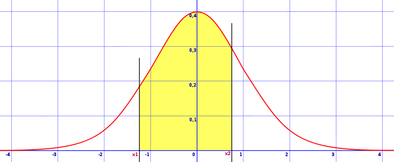
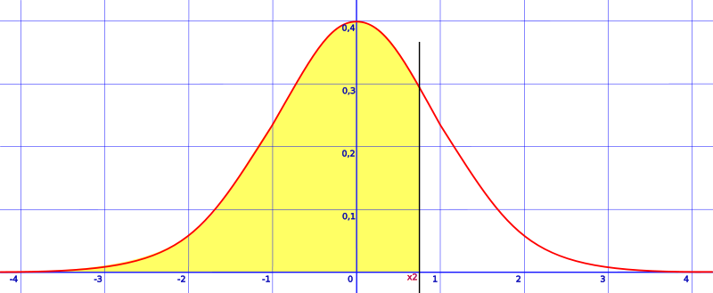
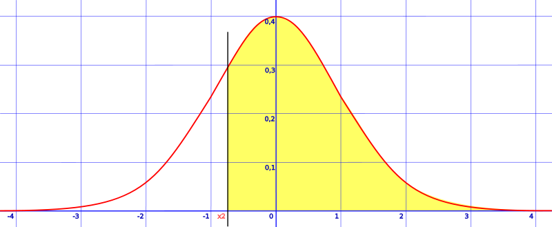
Tip: Drawing sketches in probability and statistics isn’t just limited to normal distribution curves. If you get used to making a sketch, you’ll also have an easier time with creating complicated graphs (like Contingency Table: What is it used for?.
Find an area under a normal curve from z=0 to z=?

How to find the area under a curve (between 0 and any z-score)
You can look up numbers in the z-table, like 0.92 or 1.32. The values you get from the table give you How to Calculate Percentages: Simple Steps for the area under a curve in decimal form. For example, a table value of .6700 is are area of 67%.
Note on using the table: In order to look up a z-score in the table, you have to split up your z-value at the tenths place. For example, to look up 1.32 you would look up 1.3 and then look at .02. See the example below for a visual on what finding the intersection looks like. If you need more help, watch the video on this z-table page.

Step 1: Look in the z-table for the given z-score by finding the intersection. For example, if you are asked to find the area between 0 and 0.46, look up 0.46.* The table below illustrates the result for 0.46 (0.4 in the left hand column and 0.06 in the top row. the intersection is .1772).
| z | 0.00 | 0.01 | 0.02 | 0.03 | 0.04 | 0.05 | 0.06 | 0.07 | 0.08 | 0.09 |
|---|---|---|---|---|---|---|---|---|---|---|
| 0.0 | 0.0000 | 0.0040 | 0.0080 | 0.0120 | 0.0160 | 0.0199 | 0.0239 | 0.0279 | 0.0319 | 0.0359 |
| 0.1 | 0.0398 | 0.0438 | 0.0478 | 0.0517 | 0.0557 | 0.0596 | 0.0636 | 0.0675 | 0.0714 | 0.0753 |
| 0.2 | 0.0793 | 0.0832 | 0.0871 | 0.0910 | 0.0948 | 0.0987 | 0.1026 | 0.1064 | 0.1103 | 0.1141 |
| 0.3 | 0.1179 | 0.1217 | 0.1255 | 0.1293 | 0.1331 | 0.1368 | 0.1406 | 0.1443 | 0.1480 | 0.1517 |
| 0.4 | 0.1554 | 0.1591 | 0.1628 | 0.1664 | 0.1700 | 0.1736 | 0.1772 | 0.1808 | 0.1844 | 0.1879 |
| 0.5 | 0.1915 | 0.1950 | 0.1985 | 0.2019 | 0.2054 | 0.2088 | 0.2123 | 0.2157 | 0.2190 | 0.2224 |
That’s it!
*Note. Because the graphs are symmetrical, you can ignore the negative z-scores and just look up their positive counterparts. For example, if you are asked for the area of 0 to -0.46, just look up 0.46.
Check out our YouTube channel for hundreds of statistics help videos!
References
Beyer, W. H. CRC Standard Mathematical Tables, 31st ed. Boca Raton, FL: CRC Press, pp. 536 and 571, 2002.
Agresti A. (1990) Categorical Data Analysis. John Wiley and Sons, New York.
Everitt, B. S.; Skrondal, A. (2010), The Cambridge Dictionary of Statistics, Cambridge University Press.
Gonick, L. (1993). The Cartoon Guide to Statistics. HarperPerennial.