You may want to read this other article first: What is Conditional Probability?
The conditional expectation (also called the conditional mean or conditional expected value) is simply the mean, calculated after a set of prior conditions has happened. Put more formally, the conditional expectation, E[X|Y], of a random variable is that variable’s expected value, calculated with respect to its conditional probability distribution. You can also say that E[X|Y] is the function of Y that is the best approximation for X (or, equally, the function of X that is the best approximation for Y).
Formula and Worked Example
Suppose we have two discrete random variables X and Y. with x ∈ Range(X), the condition expectation of Y given X = x:
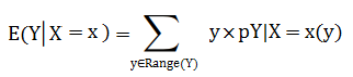
Note: X given Y = y is defined in the same way (just switch the variables).
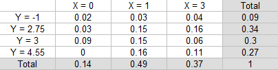
The formula might look a little daunting, but it’s actually pretty simple to work. What it is telling you to do is find the proportions of the “conditional” part (all the values where X = 1), multiply those by the Y values, then sum them all up Σ is summation notation). The process becomes much simpler if you create a joint distribution table.
Example Question: What is E(Y |X = 1)—the conditional expectation of Y, given that X = 1?
Solution:
Step 1: Find the sum of the “given” value (X = 1). This is already given in the total column of our table:
0.03 + 0.15 + 0.15 + 0.16 = 0.49.
Step 2: Divide each value in the X = 1 column by the total from Step 1:
- 0.03 / 0.49 = 0.061
- 0.15 / 0.49 = 0.306
- 0.15 / 0.49 = 0.306
- 0.16 / 0.49 = 0.327
Step 3: Multiply each answer from Step 2 by the corresponding Y value (in the left-hand column):
- 0.0612244898 * -1 = -0.061
- 0.306122449 * 2.75 = 0.842
- 0.306122449 * 3 = 0.918
- 0.3265306122 * 4.55 = 1.486
Step 3: Sum the values in Step 2:
E(Y|X = 1) = -0.061 + 0.842 + 0.918 + 1.486 = 3.19
E(Y|X = 1) = 3.19
Continuous Case
For continuous distributions, expectations must first be defined by a limiting process. The result is a function of y and x that you can interpret as a random variable. Basically, an integral represents the limiting process and replaces the sums from the example above. The formula becomes:
When we are dealing with continuous random variables, we don’t have the individual probabilities for each x that we had in the random variable example above. Instead, what you have is a probability density function for each individual x-value. To get the expected value, you integrate these pdfs over a tiny interval to essentially force the pdf to give you an approximate probability. Then, as in the steps above, you sum everything up.