What are Bernoulli Trials?

A Bernoulli trial is an experiment with two possible outcomes: Success or Failure. “Success” in one of these trials means that you’re getting the result you’re measuring. For example:
- If you flip a coin 100 times to see how many heads you get, then the Success is getting heads and a Failure is getting tails.
- You might want to find out how many girls are born each day, so a girl birth is a Success and a boy birth is a Failure.
- You want to find the probability of rolling a double six in a dice game. A double six dice roll = Success and everything else = Failure.
Note that “Success” doesn’t have the traditional meaning of triumph or prosperity. In the context of Bernoulli trials, it’s merely a way of counting the result you’re interested in. For example, you might want to know how many students get the last question on a test wrong. As you’re measuring the number of incorrect answers, the “Success” is answered incorrectly and a “Failure” is answered correctly. Of course, this might get confusing so there’s nothing stopping you tweaking your hypothesis so that you’re measuring the number of correct answers instead of incorrect ones.
Probability Distribution for Bernoulli Trials
Bernoulli trials are a special case of i.i.d. trials; Trials are i.i.d. if all the random variables in the trials have the same probability distribution.
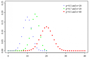
The probability distribution for a Bernoulli trial is given by the binomial probability distribution:
![]()
Where:
- ! is a factorial,
- x is the number of successes,
- n is the number of trials.
Assumptions for Bernoulli Trials
The three assumptions for Bernoulli trials are:
- Each trial has two possible outcomes: Success or Failure. We are interested in the number of Successes X (X = 0, 1, 2, 3,…).
- The probability of Success (and of Failure) is constant for each trial; a “Success” is denoted by the letter p and “Failure” is q = 1 − p.
- Each trial is independent; The outcome of previous trials has no influence on any subsequent trials.
What is Bernoulli Sampling?
Bernoulli sampling is an equal probability, without replacement sampling design. In this method, independent Bernoulli trials on population members determines which members become part of a sample. All members have an equal chance of being part of the sample. The sample sizes in Bernoulli sampling are not fixed, because each member is considered separately for the sample. The method was first introduced by statistician Leo Goodman in 1949, as “binomial sampling”.
The sample size follows a binomial distribution and can take on any value between 0 and N (where N is the size of the sample). If π is the probability of a member being chosen then the expected value (EV) for the sample size is πN. for example, let’s say you had a sample size of 100 and the probability of choosing any one item is 0.1, then the EV would be 0.1 * 100 = 10. However, the sample could theoretically be anywhere from 0 to 100.
 Example of Bernoulli Sampling: A researcher has a list of 1,000 candidates for a clinical trials. He wants to get an overview of the candidates and so decides to take a Bernoulli sample to narrow the field. For each candidate, he tosses a die: if it’s a 1, the candidate goes into a pile for further analysis. If it’s any other number, it goes into another pile that isn’t looked at. The EV for the sample size is 1/6 * 1,000 = 167.
An advantage to Bernoulli sampling is that it is one of the simplest types of sampling methods. One disadvantage is that it’s not known how large the sample is at the outset.
In SAS: Bernoulli sampling is specified with METHOD=BERNOULLI. The sampling rate is specified with the SAMPRATE= option.
In R: S.BE(N, prob) will choose a sample from population of size N with a probability of prob. For example (UPenn):
# Vector U contains the label of a population of size N=5
U <- c(“Yves”, “Ken”, “Erik”, “Sharon”, “Leslie”)
# Draws a Bernoulli sample without replacement of expected size n=3
# The inclusion probability is 0.6 for each unit in the population
sam <- S.BE(5,0.6)
sam
# The selected sample is
U[sam]
The Bernoulli Distribution
A Bernoulli Distribution is the probability an experiment produces a particular outcome. It is a binomial distribution with a single event (n = 1).
There are two variables in a Bernoulli Distribution: n and p.
- “n” represents how many times an experiment is repeated. In a Bernoulli, n = 1.
- “p” is the probability of a specific outcome happening. For example, rolling a die to get a six gives a probability of 1/6. The Bernoulli Distribution for a die landing on an odd number would be p= 1/2.
The Bernoulli and binomial distribution are often confused with each other. However, the difference between the two is slim enough for both to be used interchangeably. Technically, the Bernoulli distribution is the Binomial distribution with n=1.
Bernoulli Trial
A Bernoulli distribution is a Bernoulli trial. Each Bernoulli trial has a single outcome, chosen from S, which stands for success, or F, which stands for failure. For example, you might try to find a parking space. You are either going to be successful, or you are going to fail. Many real-life situations can be simplified to either success, or failure, which can be represented by Bernoulli Distributions.
References
Evans, M.; Hastings, N.; and Peacock, B. “Bernoulli Distribution.” Ch. 4 in Statistical Distributions, 3rd ed. New York: Wiley, pp. 31-33, 2000.
UPenn. Retrieved April 1, 2020 from: http://finzi.psych.upenn.edu/library/TeachingSampling/html/S.BE.html
Governors State University. General PPT.