Contents:
1. What is a Well Posed Problem?
A well posed problem is “stable”, as determined by whether it meets the three Hadamard criteria. These criteria tests whether or not the problem has:
- A solution: a solution (s) exists for every data point (d), for every d relevant to the problem.
- A unique solution: s is unique for all d; For every d there is at most one value of s.
- A stable solution: s depends continuously on d (a tiny change in d will lead to a tiny change in s; and a large change in d will lead to a proportionally larger change in s).
The Hadamard criteria tells us how well a problem lends itself to mathematical analysis.
Examples of Well Posedness
The majority of problems we work with in calculus, engineering, and math are well posed. That includes problems like:
- f( x ) = x2 + x,
- f( x )= 3 x / 6, and
- f( x ) = sin ( x ) + 2 x 2.
For example, take f( x ) = x 2 + x. For every real number x, x2 + x is also real and is well defined. There’s no room for ambiguity; every input k will give exactly one solution; k2 + k.
- If x = 2, f( x )= 22 + 2 or 6,
- If x = -1, f( x ) = (-1)2 – 1 = 0,
and so on.
The following continuous function is an example of a well posed function; A large difference between data points will lead to a large difference in f( x ) values, while a small difference between data points leads to a small difference in f( x ). For every a,
![]()
You can check continuity of many functions by graphing; if you don’t have to take your pencil off the paper at any point or leave any ‘ empty holes’ in your lines, the function is continuous. For more ways to test for continuity, see: How to Check the Continuity of a Function.
The History of Well Posedness
The Hadamard criteria was proposed by Jacques-Salomon Hadamard, a French mathematician, in 1923. He considered the issue of delineating between useful problems and those which weren’t worth anything scientifically. Since then we’ve discovered that many important scientific problems from a variety of fields (quantum mechanics, ultrasound testing, and optimal control theory, among other areas) can best be modeled by well posed problems.
These problems are no longer avoided and their study is an active branch of applied mathematics, but the distinctions and terminology delineating well posed and ill-posed remains the same as when Hadamard first defined it.
2. Ill-Posed Problem
An ill posed problem is one which doesn’t meet the three Hadamard criteria for being well posed. These criteria are:
- Having a solution
- Having a unique solution
- Having a solution that depends continuously on the parameters or input data.
A problem which is not well posed is considered ill posed. Many first order differential equations and inverse problems are ill posed.
For example, consider the equation y′ = ( 2 – y ) / x. The solutions of the function are y = C/x + 2, where C is a constant. Since there are an infinite number of possible values of C, there are an infinite number of solutions, and the second Hadamard criteria is not met.
Examples of Ill Posed Problems
One simple example of an ill-posed problem is given by the equation
y′ = (3/2)y1/3 with y(0) = 0.
Since the solution is y(t) = ± t3/2, the solution is not unique (it could be plus t3/2 or it could be minus t3/2). As this violates rule 2 of the Hadamard criteria, the problem is ill posed.
Many inverse problems are ill-posed because either they don’t have a solution everywhere, their solution is not unique, or their solution is not stable (continuous).
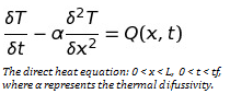 A classic example is the inverse heat problem, where the distribution of surface temperature of solid is deduced from information on the inner surface area. Although the direct heat equation (with which you can derive the interior heat from surface data) is well defined with partial derivatives, the inverse problem is not stable. The smallest changes in surface temperature data can lead to arbitrarily large differences in calculated interior heat distribution.
Hadamard and Well-Posedness
Jacques-Salomon Hadamard, the French mathematician who described the three Hadamard criteria in 1923, believed that any useful mathematical model of any physical problem must satisfy these criteria. At that time it was believed that natural problems should have continuous mathematical solutions; it was thought to be part of the inherent order of things. Since then we’ve discovered that many important scientific and technical problems are not well-posed in the traditional sense because they do not have continuous solutions.This includes problems in medicine (for instance, in Nuclear Magnetic Resonance topography and ultrasound testing), in physics (quantum mechanics, acoustics, etc.) and in economics (in optimal control theory, among other fields). Today the study of ill-posed problems is a very lively branch of applied mathematics.
Solving an Ill Posed Problem
An ill posed problem will often need to be regularized or re-formulated before you can give it a full numerical analysis using computer algorithms or other computational methods. Reformulation often involves bringing in new assumptions to fully define the problem and narrow it down.
Well Posed Problems and Tikhonov Regularization
Tikhonov Regularization (sometimes called Tikhonov-Phillips regularization) is a popular way to deal with linear discrete ill-posed problems, which violate one of the terms of a well posed problem. Regularization stabilizes ill-posed problems, giving accurate approximate solutions—often by including prior information (Vogel).
For example, let’s say you wanted to find a vector x so that Ax = b. You could use ordinary least squares to find a solution, but you may find that no solutions exist, or multiple solutions exist. Tikhonov Regularization can give you a meaningful, approximate solution to this ill-posed problem.
Tikhonov’s method can produce solutions even when the data set contains a lot of statistical noise. It is essentially the same technique as ridge regression; The main difference is that Tikhonov’s has a larger set.
The Method
Tikhobv’s method uses the following problem in place of the problem that calculates the minimum-norm least squares:
![]()
Where λ is the regularization parameter, which specifies the amount of regularization. λ essentially acts as a Lagrange multiplier, in that you are solving a minimization problem with ‖x‖ = R acting as a constraint for some R.
The basic idea is to make:
![]()
as small as possible (without minimizing it), without:
![]()
becoming too big.
More formally, the definition (from Kaipio) is:
Let λ > 0 be a given constant. The Tikhonov regularized
solution xλ ∈ H1 is
(the minimizer of the given function) provided that a minimizer exists.
The proof is beyond the scope of this site, but you can find an excellent outline in JP Kaipo’s Classical Regularization Methods (proof-of-tikhonov).
Choosing λ
Choosing a value for λ can be challenging. Several methods exist for calculating a suitable values including L-curve methods and the Morozov discrepancy principle (discussed in Kaipio).
References:
Buccini, A. Regularizing preconditioners by non-stationary iterated Tikhonov with general penalty term.
Gockenbach, M. Linear Inverse Problems and Regularization.
Kaipio, J. “Classical Regularization Methods.” Statistical and Computational Inverse Problems. Volume 160 of the series Applied Mathematical Sciences pp 7-48.
Vogel. C. Computational Methods for Inverse Problems (Frontiers in Applied Mathematics) 1st Edition.
Lecture Notes on Inverse Problems