Probability and Statistics Index > Excel for Statistics > Excel Multiple Regression
Excel multiple regression can be performed by adding a trendline, or by using the Excel Data Analysis Toolpak. If you just want to know the equation for the line of best fit, adding a trendline will work just fine. If you want to know more detailed information, like the standard error of a sample, then use the Excel Data Analysis Toolpak method.
Excel Multiple Regression: Adding a Trendline
Example question: Find the equation for the third degree polynomial that fits the following data:
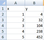
Step 1: Type your data into two columns. The x-values should be in one column (i.e. column A); the y-values should be in an adjacent column.
Step 2: Highlight both columns of data.
Step 3: Click “Insert” and then click “Scatter.” Choose the first scatter plot (Scatter with only Markers).
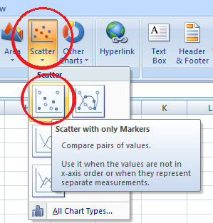
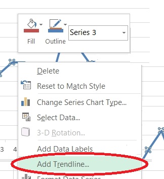
Step 4: Click on one of the data points on the graph. This will highlight all the points.
Step 5: Right click, then click “Add trendline.”
Step 6: Click the “Polynomial” radio button. Change the Order to 3.
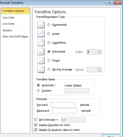
Step 7: Click “Display Equation on chart” at the bottom of the pop up window, and then press “Enter.”
Your equation will now show on the chart:
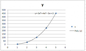
Tip: If you want to add additional significant figures to your equation’s coefficients, select the equation on the graph and then use the Number function to increase the number of decimal places.
Excel Multiple Regression: The Data Analysis Toolpak
Step 1: Type your data in (as in step 1 above).
Step 2: Add a second column containing cubes of your x-values. For this example, cube each of the x-values in column “B”.
Step 2: Click the “Data” tab and then click “Data Analysis.”
Step 3: Select BOTH columns (the x-values and their squares) when choosing x-values on the pop up window. Choose the appropriate column for the y-values.
Step 4: Check the labels box if you have column headers.
Step 5: Select the Confidence Level and Residuals boxes.
Step 6: Select an output area. Press OK.
For help with understanding what the output means, see: Excel Regression Analysis Output Explained.