Watch the video, or read on below.
Can’t see the video? Click here to watch it on YouTube.
Error propagation (or propagation of uncertainty) is what happens to measurement errors when you use those uncertain measurements to calculate something else. For example, you might use velocity to calculate kinetic energy, or you might use length to calculate area. When you use uncertain measurements to calculate something else, they propagate (grow much more quickly than the sum of the individual errors). To take this propagation into account, use one of the following formulas in your experiments.
These formulas assume your errors are random and not correlated (e.g. if you have systematic errors, you can’t use them).
Error Propagation Contents:
- Addition or Subtraction Formula
- Multiplication or Division formula
- Measured Quantity Times Exact Number formula
- General formula
- Power formula
Which formula you choose depends on how your measured quantities appear in the calculation. For example:
- Use the addition or subtraction formula if your values are added or subtracted, and the multiplication or division formula for when your quantities are multiplied or divided.
- The measured quantity × exact number should be used when multiplying by a constant with no uncertainty. For example, y =2x.
- If your formula contains multiple elements (for example, powers, additions, divisions), use the general formula.
1. Addition or Subtraction
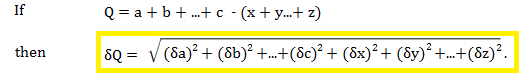
Where:
- a, b, c are positive measurements
- x, y, z are negative measurements
- δ is the error associated with each measurement (the absolute error). δa is the uncertainty associated with measurement a, δb is the uncertainty associated with measurement b, and so on.
Example of Worked Formula
Let’s say you measured your height (a) as 2.00 ± 0.03 m. Your waistband (b) is 0.88 ± 0.04 m from the top of your head, which means your pant length P would be p = H – w = 2.00 m – 0.88 m = 1.12 m.
The uncertainty, using the addition formula, is:
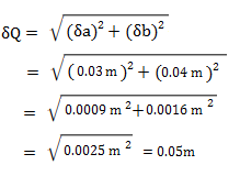
Giving a final measurement of 1.12 m ± 0.05 m.
2. Multiplication or Division formula
When calculating errors, there is no difference between multiplication and division.
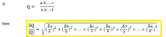
The formula looks almost the same as the addition/subtraction formula. But while Addition/Subtraction (z = x ± y) combines absolute uncertainties in quadrature, Multiplication/Division (z = x × y or x/y) combines relative uncertainties in quadrature. The subtle difference is that addition cares about raw error size (it doesn’t scale with value magnitude) while multiplication cares about percent error (it scales with size, so bigger values amplify relative errors more).
3. Power formula
If n is an exact number and Q = xn, then

Sphere volume example:
- Measure radius r = 5.0 ± 0.2, so r = 5. 0 ± 0.2 cm.
- Calculate volume V = 4/3 π r3. We have n = 3, Q = V, x = r. So, V = 4/3 π (5.0) 3 ≈ 523.6
- Calculate the power formula:
- Relative uncertainty (using the power formula): δr = 0.2/5.0 = 0.04 (4%).
- For power 3: δV/V = ∣3∣ × 0.04 = 0.12 (12%).
- For practical use, calculate the absolute uncertainty. Without it, you only have a percentage, not the actual error bars needed: δV = 0.12 × 523.6 ≈ 62.8 cm³.
4. Measured Quantity Times Exact Number formula
If A is exact measurement (e.g. A = 9 or A = π) and Q = Ax, then:
δQ = |A| δx
Length doubled example: Measure length x = 4.0 ± 0.2. We want to calculate Q = 2 x (exact factor 2, like doubling for total span).
Q = 2 x 4.0 = 8.0 cm.
δQ = |2| × δx = 2 × 0.2 = 0.4 cm.
5. General formula for Error Propagation
The general formula (using derivatives) for error propagation (from which all of the other formulas are derived) is:
![]()
Where Q = Q(x) is any function of x.
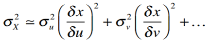
Error propagation formulas are based on taking partial derivatives of a function with respect to the variable with the uncertainty. Let’s say you had a function with three variables (x, u, v) and two of those (u, v) have uncertainty. The variance of x can be approximated by [1]:
Example question: The volume of gasoline delivered from a pump is the difference between the initial (I) and final (F) readings. If each reading has an uncertainty of ±0.02mL, what is the error in the volume delivered?
Solution:
V = F – I; σ2(V)
= σ2(I) + σ2(F)
= (0.02mL)2 + (0.02mL)2
= 0.0008mL2
= 0.028mL
The error in the volume delivered is 0.028mL.
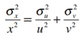
This calculation will only work when the partial derivatives are 1. The formula changes slightly when x is a product (x = uv) or quotient (x = u/v):
Example question #2: A shipping container is 12 x 10 x 8 feet with an uncertainty of 0.1ft. What is the uncertainty in the volume?
Step 1: Calculate the volume:
V = 12 x 10 x 8 = 960 ft3.
Step 2: Work the formula:
(0.1 ft)2 / (12 ft2) +
(0.1 ft)2 / (10 ft2) +
(0.1 ft)2 / (8 ft2) =
0.0003257
Step 3: Find the volume variance (Step 2 * V2):
(0.0003257)(960 ft3)2 = 0.0003257 x 921,600 = 300.46 ft6
Step 4: Take the square root of Step 3 to find the uncertainty in the volume:
√(300.46) = 17.34 ft3.
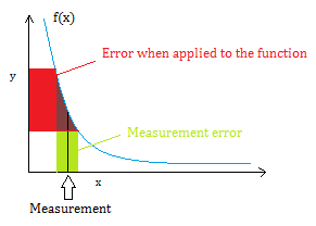
You might wonder why you can’t just add (or multiply, or divide) the errors and be done with it. Why do we have to use formulas? Very basically, one small measurement error on an independent variable, when applied to a function (say, a formula for area, kinetic energy, or velocity) is going to result in a much larger error on the dependent variable.
References
10. Error Propagation tutorial.doc. Retrieved April 14, 2021 from: https://foothill.edu/psme/daley/tutorials_files/10.%20Error%20Propagation.pdf