Statistics Definitions > Density Curve Examples
What is a Density Curve?
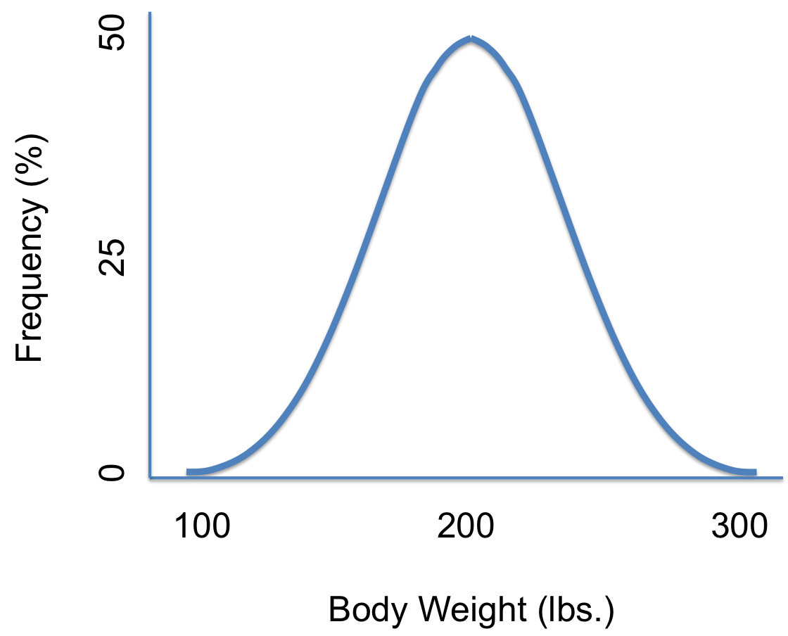
A density curve is a graph that shows probability. The area under the curve is equal to 100 percent of all probabilities. As we usually use decimals in probabilities you can also say that the area is equal to 1 (because 100% as a decimal is 1).
The above density curve is a graph of how body weights are distributed.
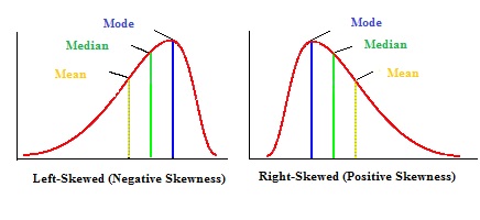
Density curves come in all shapes and sizes. They don’t have to be symmetrical distributions (like the normal distribution curve). Density curves can be a skewed distribution.
Note that the right- or left-skew doesn’t refer to how the graph looks. It refers to whether the data is skewed. Another way to think of this is that a right-skewed graph will have the mean to the right of the median, and vice versa.
Why is the Area Under a Density Curve Equal to 1?
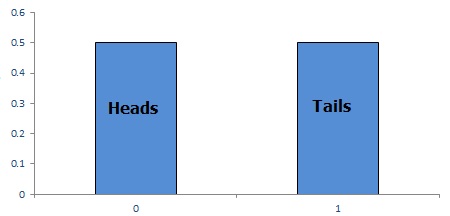
This can best be explained by using a graph with a uniform distribution. It isn’t a “curve” but the principal is the same: the area of the bars is equal to 1. The graph below is a coin toss with two bars that represent a heads or a tails. Each has an equal probability of happening (i.e. 50% or .5), which you can see on the left of the chart. The area of a rectangle is height x width, so if you multiply the height x width in this case you would get .5 x 1 = .5. Add them together and you get .5 + .5 =1.
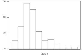
If we add more bars to the graph, like in the example histogram below, we get something that’s starting to look like a curve. If you add up all of the areas of these rectangles, they would equal 1.
With the weight density curve at the beginning of this article, you can think of it as being millions of tiny little rectangles, all adding up to get an area of 1.
For more examples of how you can use rectangles to estimate area, see: Riemann Sums.
References
Silverman, B. (1986). Density Estimation for Statistics and Data Analysis. Chapman and Hall.


