The normal approximation to the binomial is when you use a continuous distribution (the normal distribution) to approximate a discrete distribution (the binomial distribution). According to the Central Limit Theorem, the sampling distribution of the sample means becomes approximately normal if the sample size is large enough.
Normal Approximation to the Binomial: n * p and n * q Explained
Need help with a homework question? Check out our tutoring page!
The first step into using the normal approximation to the binomial is making sure you have a “large enough sample”. How large is “large enough”? You figure this out with two calculations: n * p and n * q .
- n is your sample size,
- p is your given probability.
- q is just 1 – p. For example, let’s say your probability p is .6. You would find q by subtracting this probability from 1: q = 1 – .6 = .4. Percentages (instead of decimals) can make this a little more understandable; if you have a 60% chance of it raining (p) then there’s a 40% probability it won’t rain (q).
When n * p and n * q are greater than 5, you can use the normal approximation to the binomial to solve a problem.
Normal Approximation: Example
Sixty two percent of 12th graders attend school in a particular urban school district. If a sample of 500 12th grade children are selected, find the probability that at least 290 are actually enrolled in school.
Part 1: Making the Calculations
Step 1: Find p,q, and n:
- The probability p is given in the question as 62%, or 0.62
- To find q, subtract p from 1: 1 – 0.62 = 0.38
- The sample size n is given in the question as 500
Step 2: Figure out if you can use the normal approximation to the binomial. If n * p and n * q are greater than 5, then you can use the approximation:
n * p = 310 and n * q = 190.
These are both larger than 5, so you can use the normal approximation to the binomial for this question.
Step 3: Find the mean, μ by multiplying n and p:
n * p = 310
(You actually figured that out in Step 2!).
Step 4: Multiply step 3 by q :
310 * 0.38 = 117.8.
Step 5: Take the square root of step 4 to get the standard deviation, σ:
√(117.8)=10.85
Note: The formula for the standard deviation for a binomial is √(n*p*q).
Part 2: Using the Continuity Correction Factor
Step 6: Write the problem using correct notation. The question stated that we need to “find the probability that at least 290 are actually enrolled in school”. So:
P(X ≥ 290)
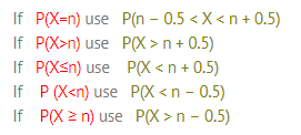
Step 7: Rewrite the problem using the continuity correction factor:
P (X ≥ 290-0.5) = P (X ≥ 289.5)
Note: The CCF table is listed in the above image, but if you haven’t used it before, you may want to view the video in the continuity correction factor article.
Step 8: Draw a diagram with the mean in the center. Shade the area that corresponds to the probability you are looking for. We’re looking for X ≥ 289.5, so:

Step 9: Find the z-score.
You can find this by subtracting the mean (μ) from the probability you found in step 7, then dividing by the standard deviation (σ):
(289.5 – 310) / 10.85 = -1.89
Step 10: Look up the z-value in the z-table:
The area for -1.89 is 0.4706.
Step 11: Add .5 to your answer in step 10 to find the total area pictured:
0.4706 + 0.5 = 0.9706.
That’s it! The probability is .9706, or 97.06%.
Check out our YouTube channel for hundreds more statistics help videos!
References
Kotz, S.; et al., eds. (2006), Encyclopedia of Statistical Sciences, Wiley.
Everitt, B. S.; Skrondal, A. (2010), The Cambridge Dictionary of Statistics, Cambridge University Press.
Vogt, W.P. (2005). Dictionary of Statistics & Methodology: A Nontechnical Guide for the Social Sciences. SAGE.
Lindstrom, D. (2010). Schaum’s Easy Outline of Statistics, Second Edition (Schaum’s Easy Outlines) 2nd Edition. McGraw-Hill Education