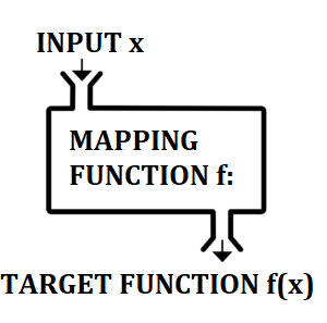
In machine learning, the mapping function takes input data and gives the corresponding output data. This gives the target function— the relationship between inputs and outputs:
Y = f(X)

The mapping function is usually a single “best” function, selected from a set of candidate functions. It is the function that best approximates the target function. However, just because it’s the top candidate from a limited selection of functions doesn’t mean that it’s a good approximation for the entire output space (Veloso & Wagner, 2011).
Mapping Function Bias Error
Mapping functions make simplifying assumptions (bias) about data before the algorithm even begins. While more assumptions can speed up the learning process, they often result in a less than optimal fit.
For example, if the data contained height and weight charts, the function might begin with the assumption that the data is normally distributed. While this can speed up the process, this restricts the algorithm to certain criteria. The algorithm is forced to constrain itself to certain parameters, so there is a chance that the data doesn’t fit the model particularly well. For example, if the population being studied was from a region suffering from famine, the normal distribution assumption would likely result in a poor fit.
Algorithms with high bias have a high number of assumptions compared to low bias algorithms. High bias algorithms include linear regression and logistic regression. On the other hand, low bias algorithms make fewer assumptions about the model. Low bias algorithms include decision trees and k-Nearest Neighbor and Support Vector Machines.
Support Vector Machine (SVM) Example Function
Exactly how the mapping function works depends on what algorithm you select. Target functions also take on many forms; Which form will depend on what process you select.
For example, an SVM’s learning process (Yan, 2015) takes a set of input data
(x1, y1), (x2, y2)…(xk, yk)
and finds a target function with a general form f(x) = (ω… x) + b.
Constraints are used during the SVM process to ensure the results are reasonable. For example, if you assume that φ(x) is a conversion function that coverts the sample data into a high-dimensional feature space, then the optimization for the algorithm can be represented by

with the following constraints:

After training, the target function can be used to find any output value (y) for any x-value outside of the training set.
References
Pathak, V. & Tiwari, P. (2018). Artificial Intelligence for All: An Abiding Destination. Educreation Publishing,
Veloso, A. & Wagner, M. (2011) Demand-Driven Associative Classification. Springer.
Yan, J. (2015). Machinery Prognostics and Prognosis Oriented Maintenance Management 1st Edition. Wiley.