Statistics Definitions > Propensity Score Matching
What is a Propensity Score?
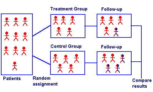
A propensity score is the probability that a unit with certain characteristics will be assigned to the treatment group (as opposed to the control group). The scores can be used to reduce or eliminate selection bias in observational studies by balancing covariates (the characteristics of participants) between treated and control groups. When the covariates are balanced, it become much easier to match participants with multiple characteristics.
What is Propensity Score Matching?
Matching designs can be bipartite, or non-bipartite. Bipartate matching is equivalent to sampling without replacement, while non-bipartate matching designs are equivalent to sampling with replacement. Bipartite designs are more common, but non-bipartite designs are available for the rare case when you want to reuse a member; For example, if you use the same control as a match for two or more treatment group participants.
Matching isn’t the only way propensity scores can be used to control confounding. Other popular methods include stratification, regression adjustment, and weighting.
Basic Steps
The basic steps to propensity score matching are:
- Collect and prepare the data.
- Estimate the propensity scores. The true scores are unknown, but can be estimated by many methods including: discriminant analysis, logistic regression, and random forests. The “best” method is up for debate, but one of the more popular methods is logistic regression.
- Match the participants using the estimated scores.
- Evaluate the covariates for an even spread across groups. The scores are good estimates for true propensity scores if the matching process successfully distributes covariates over the treated/untreated groups (Ho et. al, 2007).
Matching Algorithms
Matching methods for bipartite matching designs consist of two parts: a matching ratio and a matching algorithm. The matching ratio can be one-to-one (one from the treatment to one from the control), variable (the computer decides the optimal ratio) or fixed (each control is matched to k treatment group members). The matching algorithm is where the matching actually takes place.
One of the most popular algorithms is greedy matching, which includes caliper matching (a maximum allowable distance between propensity scores is specified) and nearest neighbor matching (matches each treatment group participant with the closest possible untreated group participant).
Other common algorithms include:
- Genetic matching: iteratively checks the propensity scores and improves them using a combination of propensity score matching and Mahalanobis distance matching (Diamond & Sekhon, 2012).
- Optimal matching: the distance between treated and untreated participants is minimized. The algorithm takes into account the entire system before making any matches (Rosenbaum, 2002).
For non-bipartite designs, the matching procedure becomes a lot more complicated. The usual algorithm is bootstrapping, which involves drawing bootstrap samples.
The matching algorithm step is usually performed with software.
- Both R (MatchIt) and SAS have procedures for optimal bipartite matching.
- Non-bipartite matching options are extremely limited, but include the nbpMatching package for R.
- The psmatch function in STATA can handle both bipartite and non-bipartite matching; It is geared to economic applications.
Criticism
The true propensity score is never known in observational studies, so you can never be certain that the propensity score estimates are accurate. Some authors urge caution in knowing the limitations of what really amounts to an estimation tool — and trying to approximate a random experiment from observational data can be fraught with pitfalls. Others, (e.g. King,2016) think that these scores shouldn’t be used for matching at all.
To avoid pitfalls, Rosenbaum & Rubin recommend iteratively checking the propensity score for balance; They provide details about the procedure in their 1983 paper. This sounds simple, but in practice it can be very challenging. Diamond and Sekhon’s genetic matching is an alternate method for achieving balance, which eliminates the need for iterative checks.
References:
Diamond, A. & Sekhon, J. (2013). Genetic Matching for Estimating Causal Effects: A General Multivariate Matching Method for Achieving Balance in Observational Studies. The Review of Economics and Statistics. July 2013, Vol. 95, No. 3, Pages: 932-945.
Ho et. al (2007). Matching as nonparametric preprocessing for reducing model dependence in parametric causal inference. Political Analysis, 15(3).
King, G. & Nielsen, R. Why prop. scores should not be used for matching. Retrieved February 2, 2017 from: http://gking.harvard.edu/files/gking/files/psnot.pdf
Rosenbaum, P. & Rubin, D. (1983). The central role of the prop. score in observational studies for causal effects. Biometricka. Apr. 1.
ROSENBAUM, P. R. (2002). Observational Studies, 2nd ed. Springer, New York. MR1899138
Image: SUNY Downstate. Retrieved August 8, 2019 from: http://library.downstate.edu/EBM2/2200.htm