Assumption of Normality > Kolmogorov-Smirnov Test
Contents:
- What is the Kolmogorov-Smirnov Test?
- How to run the test by hand
- KS Test in SPSS
- Using other software
- K-S Test P-Value Table
- Advantages and Disadvantages
- Kolmogorov-Smirnov Distribution
What is the Kolmogorov-Smirnov Test?
The Kolmogorov-Smirnov Goodness of Fit Test (K-S test) compares your data with a known distribution and lets you know if they have the same distribution. Although the test is nonparametric — it doesn’t assume any particular underlying distribution — it is commonly used as a test for normality to see if your data is normally distributed.It’s also used to check the assumption of normality in Analysis of Variance.
More specifically, the test compares a known hypothetical probability distribution (e.g. the normal distribution) to the distribution generated by your data — the empirical distribution function.
Lilliefors test, a corrected version of the K-S test for normality, generally gives a more accurate approximation of the test statistic’s distribution. In fact, many statistical packages (like SPSS) combine the two tests as a “Lilliefors corrected” K-S test.
Note: If you’ve never compared an experimental distribution to a hypothetical distribution before, you may want to read the empirical distribution article first. It’s a short article, and includes an example where you compare two data sets simply— using a scatter plot instead of a hypothesis test.
Back to top
How to run the test by hand
Need help with the steps? Check out our tutoring page!
The hypotheses for the test are:
- Null hypothesis (H0): the data comes from the specified distribution.
- Alternate Hypothesis (H1): at least one value does not match the specified distribution.
That is,
H0: P = P0, H1: P ≠ P0.
Where P is the distribution of your sample (i.e. the EDF) and P0 is a specified distribution.
General Steps
The general steps to run the test are:
- Create an EDF for your sample data (see Empirical Distribution Function for steps),
- Specify a parent distribution (i.e. one that you want to compare your EDF to),
- Graph the two distributions together.
- Measure the greatest vertical distance between the two graphs.
- Calculate the test statistic.
- Find the critical value in the KS table.
- Compare to the critical value.
Calculating the Test Statistic
The K-S test statistic measures the largest distance between the EDF Fdata(x) and the theoretical function F0(x), measured in a vertical direction (Kolmogorov as cited in Stephens 1992). The test statistic is given by:
![]()
Where (for a two-tailed test):
- F0(x) = the cdf of the hypothesized distribution,
- Fdata(x) = the empirical distribution function of your observed data.
For a one-tailed test, omit the absolute values from the formula.
If D is greater than the critical value, the null hypothesis is rejected. Critical values for D are found in the K-S Test P-Value Table.
Example
Step 1: Find the EDF. In the EDF article, I generated an EDF using Excel that I’ll use for this example.
Step 2: Specify the parent distribution. In the same article, I also calculated the corresponding values for the gamma function.
Step 3: Graph the functions together. A snapshot of the scatter graph looked like this:
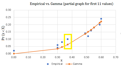
Step 4: Measure the greatest vertical distance. Let’s assume that I graphed the entire sample and the largest vertical distance separating my two graphs is .04 (in the yellow highlighted box).
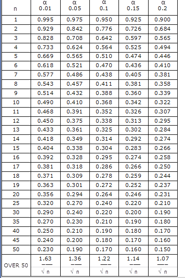
Step 5: Look up the critical value in the K-S table value. I have 50 observations in my sample. At an alpha level of .05, the K-S table value is .190.
Step 6: Compare the results from Step 4 and Step 5. Since .04 is less than .190, the null hypothesis (that the distributions are the same) is accepted.
How to Run a KS Test in SPSS
The null hypothesis for the test is that there is no significant difference between the variable and a normal distribution.
Watch the video for detailed steps:
Step 1: Analyze → descriptive statistics → explore
Step 2: Move the variables you want to test for normality over to the Dependent List box.
Step 3: (Optional if you want to check for outliers) Click Statistics, then place a check mark in the Outliers box.
Step 4: Click Plots, then place a check mark next to Histogram and Normality Plots with tests. Click Continue.
Step 5: Click Options to control how missing values should be treated.
- Exclude cases listwise: exclude any cases with missing values for the selected variables.
- Exclude cases pairwise: Compute the mean for each variable using all non-missing responses for that particular variable.
- Report values: this option will only affect analysis for a factor variable.
Click Continue.
Step 6: Click OK to run the KS Test.
Step 7: Read the results in the “Tests of Normality” section. The “Sig” column gives you your p-value. If this value is tiny (e.g., under .05 for a 5% alpha level), then you can reject the null hypothesis that the data is normally distributed. Large p-values here indicate normally distributed data.
SPSS gives you results for the Shapiro-Wilk Test at the same time. These may give you different results. You should read the K-S for large sample sizes (n ≥ 50) and the Shapiro-Wilk for small sample sizes (< 50).
The Extreme Values section will give you information about Outliers.
Using Technology
Most software packages can run this test.
The R function ecdf creates empirical distribution functions. An R function p followed by a distribution name (pnorm, pbinom, etc.) gives a theoretical distribution function.
There are several online calculators available, like this one, and this one.
As a result of using software to test for normality, small p-values in your output generally indicate the data is not from a normal distribution (Ruppert, 2004).
Back to top
K-S Test P-Value Table
Advantages and Disadvantages
Advantages include:
- The test is distribution free. That means you don’t have to know the underlying population distribution for your data before running this test.
- The D statistic (not to be confused with Cohen’s D) used for the test is easy to calculate.
- It can be used as a goodness of fit test following regression analysis.
- There are no restrictions on sample size; Small samples are acceptable.
- Tables are readily available.
Although the K-S test has many advantages, it also has a few limitations:
- In order for the test to work, you must specify the location, scale, and shape parameters. If these parameters are estimated from the data, it invalidates the test. If you don’t know these parameters, you may want to run a less formal test (like the one outlined in the empirical distribution function article).
- It generally can’t be used for discrete distributions, especially if you are using software (most software packages don’t have the necessary extensions for discrete K-S Test and the manual calculations are convoluted).
- Sensitivity is higher at the center of the distribution and lower at the tails.
What is a Kolmogorov-Smirnov Distribution?
The term “Kolmogorov Smirnov Distribution” refers to the distribution of the K-S statistic. In the vast majority of cases, the assumption is that the underlying cumulative distribution function is continuous. In those cases, the K-S distribution can be globally approximated by the general beta distribution [1].
However, some real-life applications call for a discrete distribution. While it is possible to fit a discrete distribution, working around the jump discontinuities has been problematic. In fact, there are no generally accepted efficient or exact computational methods that deal with this situation. Dimitrova et. al [2] did provide one method for a discontinuous Kolmogorov Smirnov distribution; it results in exact p-values for the test. The approach is beyond the scope of this article, but is involves expressing the complementary PDF through the rectangle probability for uniform order statistics via Fast Fourier Transform.
A K-S random variable Dn with parameter n has a cumulative distribution function of Dn −1/(2n) of [3]:

Kolmogorov-Smirnov Distribution: References
[1] Zhang, J. & Wu, Y. (2001). Beta Approximation to the Distribution of Kolmogorov-Smirnov Statistic. Ann. Inst. Statistical Math. Vol 54. No. 3, 577-584. Retrieved November 1, 2021 from: https://www.ism.ac.jp/editsec/aism/pdf/054_3_0577.pdf
[2] Dimitrova, D. et al. (2020). Computing the Kolmogorov-Smirnov Distribution When the Underlying CDF is Purely Discrete, Mixed, or Continuous. Journal of Statistical Software. Volume 95, Issue 10 (Oct). KS.
[3] Kolmogorov–Smirnov distribution. Retrieved November 15, 2021 from: http://www.math.wm.edu/~leemis/chart/UDR/PDFs/Kolmogorovsmirnov.pdf
Related Articles
References
Chakravarti, Laha, and Roy, (1967). Handbook of Methods of Applied Statistics, Volume I, John Wiley and Sons, pp. 392-394.
Ruppert, D. (2004). Statistics and Finance: An Introduction. Springer Science and Business Media.
Stephens M.A. (1992) Introduction to Kolmogorov (1933) On the Empirical Determination of a Distribution. In: Kotz S., Johnson N.L. (eds) Breakthroughs in Statistics. Springer Series in Statistics (Perspectives in Statistics). Springer, New York, NY