A plane curve is a curve in a two-dimensional plane. In other words, the points of the curve are all on the same plane. In comparison, a space curve’s points do not necessarily all lie on a single plane [1].
Plane Curve Equations
A plane curve can be defined with the parametric equation (which means that both x and y are defined as functions of a parameter, usually t) [2]
x = x(t), y = y(t),
Where coordinates (x, y) are expressed as functions of t on the closed interval t1 ≤ t ≤ t2. x(t) and y(t) are continuous functions, with a sufficient number of continuous derivatives; if there are r continuous derivatives, then the curve is class r. In vector notation, a parametric plane curve can be specified by a vector-valued function r = r(t).
The equation for a plane curve can also be expressed as rectangular coordinates f(x, y) = 0, or polar coordinates f(r, θ) = 0.
Plane curves can show a variety of interesting features, including:
- Asymptotes,
- Cusps (where a curve is tangent to itself),
- Acnodes (isolated points),
- Nodes (where the curve intersects itself).
Types of Plane Curve
The simplest plane curves arise from algebraic equations (those involving addition, subtraction, multiplication, division, roots, and raising to powers). If the curve can be described by a polynomial equation, they are called algebraic curves.
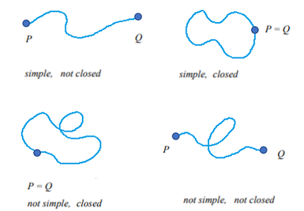
- Simple plane curves are non intersecting. In other words, they do not cross their own paths. If a curve intersects itself, then it’s not simple.
- A closed plane curve has no endpoints; it completely encloses an area. For example, a circle or ellipse; the Lamé curve is closed when n in its Cartesian equation is a positive integer. If a curve has endpoints (like a parabola), then it is an open curve.
A smooth plane curve is given by a pair of parametric equations on the closed interval [a, b]; derivatives for x(t) and y(t) exists and are continuous on [a, b] and the first derivatives are not simultaneously zero on that interval [3].
See also:
References
[1] Montoya, D. & Naves, D. On Plane and Space Curves. Retrieved January 15, 2022 from: https://web.ma.utexas.edu/users/drp/files/Spring2020Projects/DRP_Final_Project%20-%20Daniel%20Naves.pdf
[2] Patrikalakis, N. et al. (2009). 1.1.1 Plane Curves. Retrieved January 15, 2022 from: https://web.mit.edu/hyperbook/Patrikalakis-Maekawa-Cho/node5.html
[3] Length of Curve and Surface Area.
Cassini Oval
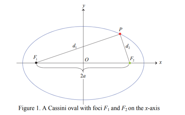
A Cassini oval is a plane curve defined as the set of points in the plane with the products of distances to two fixed points (loci) F1 and F2 is constant [1]; as a formula, the distance is (F1, F2) = 2a [2].
Cassini ovals are generalizations of lemniscates. The ovals are similar to ellipses, but instead of adding distances to loci, you multiply them.
The curve is symmetric with respect to the x-axis, the y-axis, and the origin.
Equations
The general equation is (x2 + y2 + a2)2 – 4a2x2 = b4.
The polar equation is r4 − 2a2r2cos 2θ + a4.
Cassini Oval Shapes
The ovals can take on three different shapes, shown in the following image:
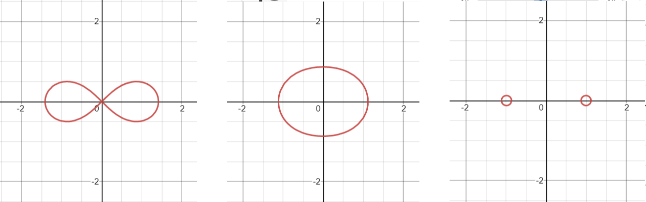
- When a = b, the oval resembles an infinity symbol ∞, which is a Leminiscate of Bernoulli.
- When a < b, the oval takes on the shape of an ellipse or peanut shell.
- If a > b, the oval splits into two ellipses shaped like eggs, with the narrow ends of the “eggs” facing each other. The shapes are mirror-images of each other.
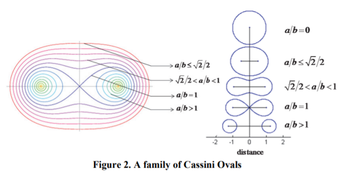
The following image shows the various shapes the Cassini oval can take on, in one image:
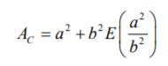
Area of Cassini Ovals
The area of a Cassini oval can be found in several ways, including numerical integration and elliptic integrals. What follows is a summary, you can find more detail on pages 235-236 of this PDF.
The oval is symmetric to both the x- and y-axes, so we can find the area of one quarter of an oval, and multiply by 4:
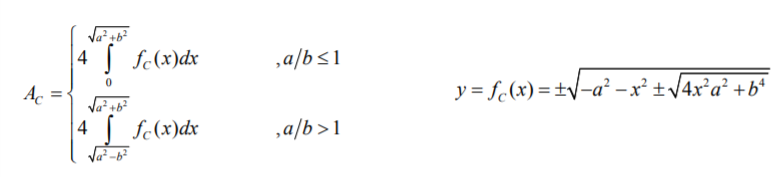
You can also calculate the area with the following elliptic integral, where E(x) is the complete elliptic integral of the second kind:
History of the Cassini Oval
Cassini ovals were first studied by 15th Century Giovanni Cassini, who used the ovals to model the sun’s orbit around the Earth [3]. The orbits of the planets around the sun, orbits of satellites around a planet, and electron orbits in atoms, can all be modeled by a Cassini Oval. This may come as a surprise; a common misconception is that planetary orbits are highly elliptical [4].
Cassini Ovals have a wide variety of uses, including developing radar and sonar systems, modeling human blood cells, and fuel tank optimization.
References
“Three different shapes” image created with Desmos.
[1] Mümtaz, K. A Multi Foci Closed Curve: Cassini Oval, Its Properties and Applications. Institutional Archive of the Naval Postgraduate School. 2013. PDF.
[2] Hellmers, J. et al. Simulation of light scattering by
biconcave Cassini ovals using the nullfield method with discrete sources. Journal of
Optics A: Pure and Applied Optics, Pure Appl. Opt. Vol 8. pp. 1-9. 2006.
[3] Gibson, K. The ovals of Cassini. Lecture Notes. 2007. Retrieved February 11, 2012 from: https://mse.redwoods.edu/darnold/math50c/CalcProj/sp07/ken/CalcPres.pdf
[4] Morgado, B. & Soares, V. Kepler’s ellipse, Cassini’s oval and the trajectory of planets. Eur. J. Phys. 35 (2014) 025009.