Regression Analysis > Simultaneous Equations Model (SEM)
You may want to read this other article first: What is Simultaneity?
What is a Simultaneous Equations Model (SEM)?
A Simultaneous Equation Model (SEM) is a model in the form of a set of linear simultaneous equations. Where introductory regression analysis introduces models with a single equation (e.g. simple linear regression), SEM models have two or more equations. In a single-equation model, changes in the response variable (Y) happen because of changes in the explanatory variable (X); in an SEM model, other Y variables are among the explanatory variables in each SEM equation. The system is jointly determined by the equations in the system; In other words, the system exhibits some type of simultaneity or “back and forth” causation between the X and Y variables.
SEM Example
The market for graduate nurses is influenced by:
- Demand behavior,
- Supply behavior,
- Equilibrium levels for pay rate and employment.
Let’s say that the simultaneous equations model for this scenario is made up the following two equations**:
- Demand: nt = β1 + β2gt + β3pt + ε1t
- Supply: nt = β11 + β12mt + β13pt + ε2t
Where:
- n = number of employed nurses,
- p = earnings rate,
- g = graduate nursing school enrollment,
- m = median income for employed nurses.
**These formulas are just regression equations tailored for this specific model; β is the regression coefficient and ε is the error term — unexpected factors that can creep into the model.
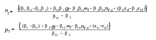
Using the Model to Solve Problems
Remember those simultaneous equations from algebra? They can be solved together to find values for x and y. In the same way, the equations in SEM can also be solved. Using the above example, let’s say you wanted to find out the partial impact of median pay (m) on both the number of employed nurses (n) and the pay rate (p). You can model this by solving the equations for n and p:
Complete Models and Structural Equation Models
When the total number of endogenous variables is equal to the number of equations, it is called a complete SEM. Endogenous variables are similar to (but not exactly the same as) dependent variables; They have values that are determined by other variables in the system (these “other” variables are called exogenous variables). If earnings rate and number of employed nurses are the only two endogenous variables in the above example, then this SEM is complete. A complete SEM is called a structural equations model.
Structural Equation Modeling and Relationship to Simultaneous Equations Models
The terms structural equation modeling and simultaneous equations modeling are similar — and often confused — but they are not exactly the same thing. Underpinning any statistical modeling technique is a set of simultaneous equations. Structural equation models use these equations and are complete Simultaneous Equations Models. “Complete” means that the total number of endogenous variables is equal to the number of equations in the model. In other words, if the number of endogenous variables in your model doesn’t equal the number of equations, then it is not a structural equation model.
The primary variables used in Structural Equation Modeling are usually latent variables, which are compared with observed variables in the model. A latent or “hidden” variable is not directly measurable or observable. For example, a person’s level of neurosis, conscientiousness or openness are all latent variables. Latent variables are ever-present in nearly all regression analysis, because all additive error terms are not measurable (and are therefore latent).
In some specific cases structural equation modeling is used to create a model; One of the most common modeling techniques — Regression Analysis — is a special case of Structural Equation Modeling.
Three Modeling Techniques
Structural Equation Modeling is a general term for a set of three modeling techniques in statistics. It is usually used to confirm that a chosen model is valid. In other words, it’s used to test if a model accurately represents sample data. Unlike the bulk of statistical techniques, structural equation modeling can handle complex theoretical relationships between multiple sets of variables. This technique also takes measurement error into account, something which basic statistical techniques do not do.
Structural Equation Models look for relationships between sets of latent variables. First developed in the latter half of the 20th century by Karl G. Jöreskog, it combines path analysis and confirmatory factor analysis. The three techniques included in the umbrella term Structural Equation Modeling are:
- Regression analysis only deals with observed variables. In regression, one dependent variable is predicted using a set of independent variables. For example, a patient’s weight is used to predict their risk for diabetes. Regression is one of the earliest modeling techniques and was made possible after Karl Pearson’s development of the correlation coefficient.
- Path analysis , developed by biologist Sewell Wright in the early 1900s, can use observed variables or a combination of observed and latent variables. Very basically, a path model is regression analysis with latent variables. For example, you might want to predict how interest rates and GNP influence consumer spending and consumer trust.
- Factor Analysis looks for relationships between sets of latent variables (“factors”). It can answer questions like “Does my ten question survey accurately measure one specific factor?”. Spearman (1904) was the first person to use the term Factor Analysis; he used it to find a two-factor construct for intelligence. Later, Confirmatory Factor Analysis was developed to test if a set of latent variables accurately depicted a construct. Latent Class Analysis is very similar; the main difference is that LCA includes categorical dependent variables and Factor Analysis does not.
Next: Index of Fit
References:
C. Spearman. “General Intelligence,” Objectively Determined and Measured. The American Journal of Psychology. Vol. 15, No. 2 (Apr., 1904), pp. 201-292
Karl G. Jöreskog. Structural equation modeling with ordinal variables. Lecture Notes–Monograph Series. Volume 24, 1994, 297-310.
Randall E. Schumacker, Richard G. Lomax. A Beginner’s Guide to Structural Equation Modeling: Fourth Edition