Sign Test: Step by Step Calculation

What is the Sign Test?

The sign test compares the sizes of two groups. It is a non-parametric or “distribution free” test, which means the test doesn’t assume the data comes from a particular distribution, like the normal distribution. The sign test is an alternative to a one sample t test or a paired t test. It can also be used for ordered (ranked) categorical data.

The null hypothesis for the sign test is that the difference between medians is zero.

For a one sample sign test, where the median for a single sample is analyzed, see: One Sample Median Tests.

How to Calculate a Paired/Matched Sample Sign Test

Assumptions for the test (your data should meet these requirements before running the test) are:

The data should be from two samples.
The two dependent samples should be paired or matched. For example, depression scores from before a medical procedure and after.

To set up the test, put your two sets of sample data into a table (I used Excel). This set of data represents test scores at the end of Spring and the beginning of the Fall semesters. The hypothesis is that the summer break means a significant drop in test scores.

H₀: No difference in median of the signed differences.
H₁: Median of the signed differences is less than zero.

Step 1: Subtract set 2 from set 1 and put the result in the third column.

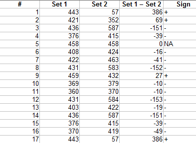
Step 2: Add a fourth column indicating the sign of the number in column 3.

Step 3: Count the number of positives and negatives.

4 positives.
12 negatives.

12 negatives seems like a lot, but we can’t say for sure that it’s significant (i.e. that it didn’t happen by chance) until we run the sign test.

Step 3: Add up the number of items in your sample and subtract any you had a difference of zero for (in column 3). The sample size in this question was 17, with one zero, so n = 16.

Step 4: Find the p-value using a binomial distribution table or use a binomial calculator. I used the calculator, putting in:

.5 for the probability. The null hypothesis is that there are an equal number of signs (i.e. 50/50). Therefore, the test is a simple binomial experiment with a .5 chance of the sign being negative and .5 of it being positive (assuming the null hypothesis is true).
16 for the number of trials.
4 for the number of successes. “Successes” here is the smaller of either the positive or negative signs from Step 2.

The p-value is 0.038, which is smaller than the alpha level of 0.05. We can reject the null hypothesis and say there is a significant difference.

References

Kotz, S.; et al., eds. (2006), Encyclopedia of Statistical Sciences, Wiley.
Lindstrom, D. (2010). Schaum’s Easy Outline of Statistics, Second Edition (Schaum’s Easy Outlines) 2nd Edition. McGraw-Hill Education
Vogt, W.P. (2005). Dictionary of Statistics & Methodology: A Nontechnical Guide for the Social Sciences. SAGE.
Wheelan, C. (2014). Naked Statistics. W. W. Norton & Company