Contents (click to skip to that section):
- What is a Sampling Distribution?
- Mean of the sampling distribution of the mean
- Mean of Sampling Distribution of the Proportion
- Standard Deviation of Sampling Distribution of the Proportion
Definition
Watch the video for an overview:
A sampling distribution is a graph of a statistic for your sample data. While, technically, you could choose any statistic to paint a picture, some common ones you’ll come across are:
- Mean
- Mean absolute value of the deviation from the mean
- Range
- Standard deviation of the sample
- Unbiased estimate of variance
- Variance of the sample
Up until this point in statistics, you’ve probably been plotting graphs for a set of numbers. For example, you might have graphed a data set and found it follows the shape of a normal distribution with a mean score of 100. Where probability distributions differ is that you aren’t working with a single set of numbers; you’re dealing with multiple statistics for multiple sets of numbers. If you find that concept hard to grasp: you aren’t alone.
While most people can imagine what the graph of a set of numbers looks like, it’s much more difficult to imagine what stacks of, say, averages look like.
An explanation…
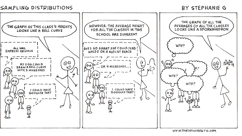
Let’s start with a mean, like heights of students in the above cartoon. As you probably know, heights (and many other natural phenomenon) follow a bell curve shape. So if you surveyed your class, you’d probably find a few short people, a few tall people, and most people would fall in between. Let’s say the average height was 5’9″. Survey all the classes in your school and you’ll probably get somewhere close to the average. If you had 10 classes of students, you might get 5’9″, 5’8″, 5’10”, 5’9″, 5’7″, 5’9″, 5’9″, 5’10”, 5’7″, and 5’9″. If you graph all of those averages, you’re probably going to get a graph that resembles the “sporkahedron.” For other data sets, you might get something that looks flatlined, like a uniform distribution. It’s almost impossible to predict what that graph will look like, but the Central Limit Theorem tells us that if you have a ton of data, it’ll eventually look like a bell curve. That’s the basic idea: you take your average (or another statistic, like the variance) and you plot those statistics on a graph.
This video introduces the Central Limit Theorem as it applies to these distributions. The “mean of the sampling distribution of the means” is just math-speak for plotting a graph of averages (like I outlined above) and then finding the average of that set of data.
Mean of the sampling distribution of the mean
In a nutshell, this is the same as the population mean. For example, if your population mean (μ) is 99, then the mean of the sampling distribution of the mean, μm, is also 99 (as long as you have a sufficiently large sample size). If you want to understand why, watch the video or read on below.
The Central Limit Theorem.
Roughly stated, the central limit theorem tells us that if we have a large number of independent, identically distributed variables, the distribution will approximately follow a normal distribution. It doesn’t matter what the underlying distribution is.
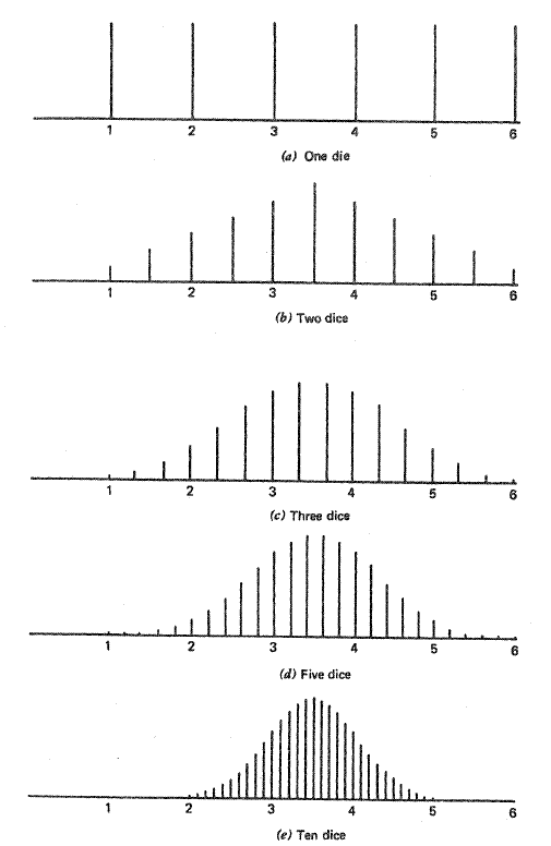
Here’s a simple example of the theory: when you roll a single die, your odds of getting any number (1,2,3,4,5, or 6) are the same (1/6). The mean for any roll is (1 + 2 + 3 + 4 + 5 + 6) / 6 = 3.5. The results from a one-die roll are shown in the first figure below: it looks like a uniform distribution. However, as the sample size is increased (two dice, three dice…), the distribution of the mean looks more and more like a normal distribution. That is what the central limit theorem predicts.
As the sample size increases, distribution of the mean will approach the population mean of μ, and the variance will approach σ2/N, where N is the sample size.
You can think of a sampling distribution as a relative frequency distribution with a large number of samples.
The mean of the sampling distribution of the mean formula
The formula is μM = μ, where μM is the mean of the sampling distribution of the mean.
Mean of Sampling Distribution of the Proportion
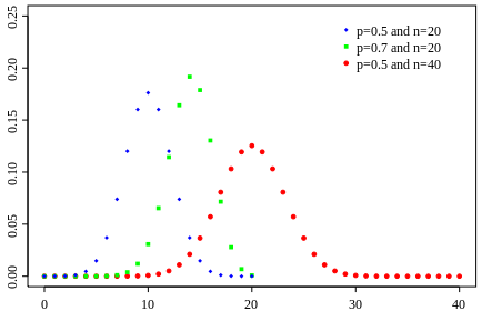
The mean of sampling distribution of the proportion, P, is a special case of the sampling distribution of the mean. The mean of the sampling distribution of the proportion is related to the binomial distribution.
Proportions are something you probably already know. For example: 100 people are asked if they are democrat. If 50 people respond “yes” then the sample proportion p = 50/100. Technically (the “mathy way”): A sample proportion is where a random sample of objects n is taken from a population P; if x objects have a certain characteristic then the sample proportion “p” is: p = x/n.
The sampling distribution of a proportion is when you repeat your survey or poll for all possible samples of the population. For example: instead of polling asking 1000 cat owners what cat food their pet prefers, you could repeat your poll multiple times.
Mean of Sampling Distribution of the Proportion
If a random sample of n observations is taken from a binomial population with parameter p, the sampling distribution (i.e. all possible samples taken from the population) will have a mean up=p. With a large sample, the sampling distribution of a proportion will have an approximate normal distribution.
Standard Deviation of Sampling Distribution of the Proportion
The standard deviation of sampling distribution of the proportion, P, is also closely related to the binomial distribution and is a special case of a sampling distribution.
Example: You hold a survey about college student’s GRE scores and calculate that the standard deviation is 1. It is highly unlikely that you will get the same results if you repeat the survey (you might get 1.1 ,1.2 or 0.9). Therefore you’ll want to repeat the poll the maximum number of times possible (i.e. you draw all possible samples of size n from the population). You’ll have a range of standard deviations — one for each sample.
Sampling Distribution of a Proportion
This is when you repeat your survey for all possible samples of the population. For example: instead of polling 100 people once to ask if they are democrat, you’ll poll them multiple times to get a better estimate of your statistic.
Standard Deviation
If a random sample of n observations is taken from a binomial population with parameter p, the sampling distribution (i.e. all possible samples taken from the population) will have a standard deviation of:
Standard deviation of binomial distribution = σp = √[pq/n] where q=1-p.
When the sample is large, the distribution will have an approximate normal distribution.
Check out our YouTube channel for more tips and help for stats!
References
Everitt, B. S.; Skrondal, A. (2010), The Cambridge Dictionary of Statistics, Cambridge University Press.
Gonick, L. (1993). The Cartoon Guide to Statistics. HarperPerennial.
Kotz, S.; et al., eds. (2006), Encyclopedia of Statistical Sciences, Wiley.
Levine, D. (2014). Even You Can Learn Statistics and Analytics: An Easy to Understand Guide to Statistics and Analytics 3rd Edition. Pearson FT Press