Statistics Definitions > Heteroscedasticity
The word “heteroscedasticity” comes from the Greek, and quite literally means data with a different (hetero) dispersion (skedasis). In simple terms, heteroscedasticity is any set of data that isn’t homoscedastic. More technically, it refers to data with unequal variability (scatter) across a set of second, predictor variables.
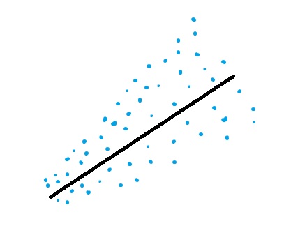
Why do we care about whether or not data is heteroscedastic? Most of the time in statistics, we don’t care. But if you’re running any kind of regression analysis, having data that shows heteroscedasticity can ruin your results (at the very least, it will give you biased coefficients). Therefore, you’ll want to check to make sure your data doesn’t have this condition. One way to check is to make a scatter graph (which is always a good idea when you’re running regression anyway). If your graph has a rough cone shape (like the one above), you’re probably dealing with heteroscedasticity. You can still run regression analysis, but you won’t get decent results.
In regression, an error is how far a point deviates from the regression line. Ideally, your data should be homoscedastic (i.e. the variance of the errors should be constant). Outside of classroom examples, this situation rarely happens in real life. Most data is heteroscedastic by nature. Take, for example, predicting women’s weight from their height. In a Stepford Wives world, where everyone is a perfect dress size 6, this would be easy: short women weigh less than tall women. But in the real world, it’s practically impossible to predict weight from height. Younger women (in their teens) tend to weigh less, while post-menopausal women often gain weight. But women of all shapes and sizes exist over all ages. This creates a cone shaped graph for variability.
Plotting variation of women’s height/weight would result in a funnel that starts off small and spreads out as you move to the right of the graph. However, the cone can be in either direction (left to right, or right to left):
- Cone spreads out to the right: small values of X give a small scatter while larger values of X give a larger scatter with respect to Y.
- Cone spreads out to the left: small values of X give a large scatter while larger values of X give a smaller scatter with respect to Y.
Heteroscedasticity can also be found in daily observations of the financial markets, predicting sports results over a season, and many other volatile situations that produce high-frequency data plotted over time.
How to Detect Heteroscedasticity
A residual plot can suggest (but not prove) heteroscedasticity. Residual plots are created by:
- Calculating the square residuals.
- Plotting the squared residuals against an explanatory variable (one that you think is related to the errors).
- Make a separate plot for each explanatory variable you think is contributing to the errors.
You don’t have to do this manually; most statistical software (i.e. SPSS, Maple) have commands to create residual plots.
Several tests can also be run:
Consequences of Heteroscedasticity
Severe heteroscedastic data can give you a variety of problems:
- OLS will not give you the estimator with the smallest variance (i.e. your estimators will not be useful).
- Significance tests will run either too high or too low.
- Standard errors will be biased, along with their corresponding test statistics and confidence intervals.
How to Deal with Heteroscedastic Data
If your data is heteroscedastic, it would be inadvisable to run regression on the data as is. There are a couple of things you can try if you need to run regression:
- Give data that produces a large scatter less weight.
- Transform the Y variable to achieve homoscedasticity. For example, use the Box-Cox normality plot to transform the data.