Fractile: Simple Definition

Statistics Definitions >

A fractile is the cut off point for a certain fraction of a sample. If your distribution is known, then the fractile is just the cut-off point where the distribution reaches a certain probability.

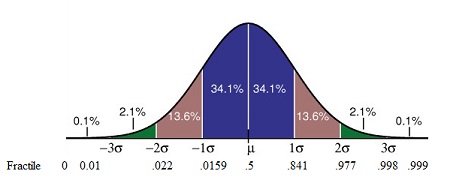
In visual terms, a fractile is the point on a probability density curve (PDF) so that the area under the curve between that point and the origin (i.e. zero) is equal to a specified fraction. For example, a fractile of .25 cuts off the bottom quarter of a sample and .5 cuts the sample in half. The following image shows the PDF for a normal distribution along with standard deviations (σ) and associated fractiles.

A fractile x_p for p greater than 0.5 is called an upper fractile, and a fractile x_p for p less than 0.5 is called a lower fractile.

Fractiles are important in engineering and scientific applications, and a different form of them– percentiles, see below– are one of the first real life exposure many of us get to statistics, as our parents look up the growth percentiles of our baby siblings and we look up the percentile our SAT scores fall in.

Quantiles, Quartiles, Deciles and Percentiles

The word quantile is sometimes used instead of the word fractile, and they can be expressed as quartiles, deciles, or percentiles by expressing the decimal or fraction α in terms of quarters, tenths, or hundredths respectively.

The 1/4-frac x_0.25 is the same as the 1st quartile. The 1/2-frac is the 2nd-quartile, and the 3/4-frac is the 3rd quartile.

In the same way, the 0.10-frac is the first decile, the 0.40-frac the fourth decile, and so on.

The 0.01 frac is the first percentile, the 0.23 frac the 23rd percentile, and the 0.99 fract the 99th percentile.

Terminology

More precisely, for a continuous distribution of a random variable we can define α fractile (x_α) to be that point on the distribution such that the variable X has a probability α of being less than or equal to the point.

Symbolically, we can define the fractile x_p by writing
P(X ≤ x_p)= Φ (x_p) = p .

Here φ (x) is the distribution function of your random variable X. Looking at the fractile of 0.8441 in the image above, P(X ≤ (μ + σ) )= φ (μ + σ)) = 0.8441, so x_p = μ + σ. If your distribution has a mean of 6 and a standard deviation of 2, the fractile of 0.8441 will be 8 and the fractile of 0.5 = 6.

Calculations

A fractile is just a cut-off point for a certain probability, so if your distribution is known then you can just look it up in the relevant table. For example, the z-table shows these cut-off points (x_p) for the normal distribution.
You can calculate the x_p of your non-standard random variable X from the fractile u_p using the standardized variable U with the following formula:

.
Where:

• V is the coefficient of variation for your variable X.  
• μ is the mean
• σ is the standard deviation
• u_p is the fractile of the standardized normal variable corresponding to probability p. For example, u_0.1 corresponds to p = .1

In order to find u_p, consult a table for the specific distribution you’re working with. For example, the following table shows u_p of a standardized random variable with a normal distribution (from Milan Holický’s Introduction to Probability and Statistics for Engineers).


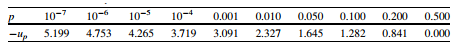
For example, suppose you wanted to calculate the value of x_p for p = 0.10 where the coefficient of variability was 0.3 and the mean 5. u_p is 1.282, so x_p will be 5(1 + 1.282 · 0.3) or 6.923.

Calculating fractiles for variables when you don’t know the underlying distribution can be tricky. Three methods are available: classical coverage method, prediction method, and a Bayesian approach. These advanced tools are usually used by engineers and can be found in the relevant International Organization for Standardization (ISO) publications. For example, classical coverage is outlined in ISO 12491.

• The classical coverage method obtains values within a certain confidence interval, rather than an exact figure. Although this method can work with very small sample sizes, skewness must be known from prior experience.
• The prediction method, prediction limits are used as a constraint for new values.
• The Bayesian approach uses prior knowledge for distributions of random variables.

More details about these three methods can be found in Holický’s Introduction to Probability and Statistics for Engineers.

References

Agarwal, B. Basic Statistics. Anshan Publishers, 2012.
Holicky, M. Introduction to Probability and Statistics for Engineers. Springer Science & Business Media, 2013.
Madsen B. Statistics for Non-Statisticians. Springer Science & Business Media. 2011.