Sampling > Finite Population Correction Factor
What is the Finite Population Correction Factor?
The Finite Population Correction Factor (FPC) is used when you sample without replacement from more than 5% of a finite population. It’s needed because under these circumstances, the Central Limit Theorem doesn’t hold and the standard error of the estimate (e.g. the mean or proportion) will be too big. In basic terms, the FPC captures the difference between sampling with replacement and sampling without replacement.
Most real-life surveys involve finite populations sampled without replacement. For example, you might perform a telephone survey of 10,000 people; once a person has been called, they won’t be called again.
Note: A downside of using the FPC is that it can cause uncertainty when applying the results to a larger population, so you should be careful when making inferences.
Formula
The general formula is:
Where:
- N = population size,
- n = sample size.
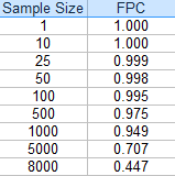
If the calculated value for the FPC is close to 1, it can be ignored. As the sample size falls under 5%, the value becomes somewhat insignificant (an FPC is .998 for a sample of 50).
The following table of values shows how the FPC decreases for a population of 10,000 as the sample size gets larger:
How to Use the Formula
Basically, place the correction at the end of the formula you want to use. For example, the standard error of the mean formula is:
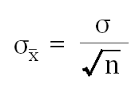
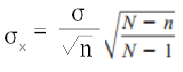
And with the correction, the formula is:
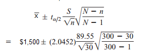
Or, for a confidence interval for a mean and unknown population standard deviation, the formula (with FPC) is: ![]()
Example
Thirty people from a population of 300 were asked how much they had in savings. The sample mean (x̄) was $1,500, with a sample standard deviation of $89.55. Construct a 95% confidence interval estimate for the population mean.
Solution (using degrees of freedom = n – 1 = 29) and tα/2 = 2.0452 for a 95% confidence level):
= $1,500 ± 33.44(0.9503)
= $1,500 ± 31.776
= $1,468.22 ≤ μ ≤ $1,531.78.
References:
Kandethody, M. et, al. Mathematical Statistics with Applications. Elsevier India (2012). p.187.