Dixon’s Q Test: Definition, Step by Step Examples + Q Critical Values Tables

Find Outliers > Dixon’s Q Test

What is Dixon’s Q Test?

Dixon’s Q test, or just the “Q Test” is a way to find outliers in very small, normally distributed, data sets. Small data sets are usually defined as somewhere between 3 and 7 items. It’s commonly used in chemistry, where data sets sometimes include one suspect observation that’s much lower or much higher than the other values. Keeping an outlier in data affects calculations like the mean and standard deviation, so true outliers should be removed.

Dixon came up with many different equations to find true outliers. The most commonly used one is called the R₁₀ or simply the “Q” version, which is used to test if one single value is an outlier in a sample size of between 3 and 7. Dean and Dixon did suggest various other formulas in a later paper, but these are not commonly used. For a full list of alternate formulas for different sample sizes (up to about 30), go to: Dixon’s Test, Alternate Formulas and Tables.

How to Run Dixon’s Q Test (R₁₀).

Note: make sure your data set is normally distributed before running the test; for example, run a Shapiro-Wilk test. Running it on different distributions will lead to erroneous results. An extreme value may throw off any test for normality, so try running that test without the suspect data item. If your data set still doesn’t meet the assumption of normality after running a test for it, then you should not run Dixon’s Q Test,

Caution: the test should not be used more than once for the same set of data.

Example:: Is 167 an outlier in this set of data? Test at the 95% confidence Level (i.e. at an alpha level of 5%).
167, 180, 188, 177, 181, 185, 189

Step 1: Sort your data into ascending order (smallest to largest).
167, 177, 180, 181, 185, 188, 189.

Step 2 :Find the Q statistic using the following formula:



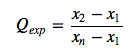
Where:

• x₁ is the smallest (suspect) value,
• x₂ is the second smallest value,
• and x_n is the largest value.

Inserting the values into the formula, we get:
Q = (177 – 167) / 189 – 167 = 10/22 = 0.455.

Step 3: Find the Q critical value in the Q table (scroll to the bottom of the article for the table). For a sample size of 7 and an alpha level of 5%, the critical value is 0.568.

Step 4: Compare the Q statistic from Step 2 with the Q critical value in Step 3. If the Q statistic is greater than the Q critical value, the point is an outlier.
Q_statistic = 0.455.
Q_{critical value} = 0.568.

Solution: 0.455 is not greater than 0.568, so this point is not an outlier at an alpha level of 5%.

Dixon’s Q Table

This table shows the more common Alpha Levels .10, .05 and .01. You can find less common alpha levels on the UC Davis website.

Sample size:	3	4	5	6	7	8	9	10
α = .10:	0.941	0.765	0.642	0.560	0.507	0.468	0.437	0.412
α = .05:	0.970	0.829	0.710	0.625	0.568	0.526	0.493	0.466
α = .01:	0.994	0.926	0.821	0.740	0.680	0.634	0.598	0.568

Dixon’s Test, Alternate Formulas and Tables.

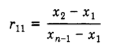
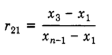
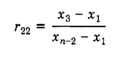
Finding the Q statistic for different sample sizes (n) of between 8 and 30 (in Step 2 above):
8< n >10: use R₁₁:



11< n >13: use R₂₁.


14< n >30: use R₂₂.

Q critical values for r₁₁

N	α = 0.001	α = 0.002	α = 0.005	α = 0.01	α = 0.02	α = 0.05	α = 0.1	α = 0.2
8	0.799	0.769	0.724	0.682	0.633	0.554	0.480	0.386
9	0.750	0.720	0.675	0.634	0.586	0.512	0.441	0.352
10	0.713	0.683	0.637	0.597	0.551	0.477	0.409	0.325

Q critical values for r₂₁

N	α = 0.001	α = 0.002	α = 0.005	α = 0.01	α = 0.02	α = 0.05	α = 0.1	α = 0.2
11	0.770	0.746	0.708	0.674	0.636	0.575	0.518	0.445
12	0.739	0.714	0.676	0.643	0.605	0.546	0.489	0.420
13	0.713	0.687	0.649	0.617	0.580	0.522	0.467	0.399

Q critical values for r₂₂

N	α = 0.001	α = 0.002	α = 0.005	α = 0.01	α = 0.02	α = 0.05	α = 0.1	α = 0.2
14	0.732	0.708	0.672	0.640	0.603	0.546	0.491	0.422
15	0.708	0.685	0.648	0.617	0.582	0.524	0.470	0.403
16	0.691	0.667	0.630	0.598	0.562	0.505	0.453	0.386
17	0.671	0.647	0.611	0.580	0.545	0.489	0.437	0.373
18	0.652	0.628	0.594	0.564	0.529	0.475	0.424	0.361
19	0.640	0.617	0.581	0.551	0.517	0.462	0.412	0.349
20	0.627	0.604	0.568	0.538	0.503	0.450	0.401	0.339
25	0.574	0.550	0.517	0.489	0.457	0.406	0.359	0.302
30	0.539	0.517	0.484	0.456	0.425	0.376	0.332	0.278

 

Reference:
R. B. Dean and W. J. Dixon (1951) Simplified Statistics for Small Numbers of Observations. Anal. Chem., 1951, 23 (4), 636–638. Found online here.
Rorabacher, David B. (1991) Statistical Treatment for Rejection of Deviant Values: Critical Values of Dixon’s‘ Q’ Parameter and Related Subrange Ratios at the 95% Confidence Level. Analytical Chemistry 63, no. 2 (1991): 139–46. Found online here.